4.2.9.1 Statement 2: Hamiltonian maximization condition

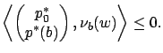
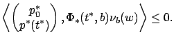
Let us go back to the formula (4.23), which says that the infinitesimal perturbation of the terminal point caused by a needle perturbation of the optimal control with parameters $w$ , $b$ , $a$ is described by the vector $\varepsilon \Phi_*(t^*,b)\nu_b(w)a$ . This vector was subsequently labeled as $\varepsilon \delta(w,I)$ , and by construction $y^*(t^*)+\varepsilon \delta(w,I)$ belongs to the terminal cone $C_{t^*}$ . Applying the inequality (4.29) which encodes the separating hyperplane property, and noting that $\varepsilon$ and $a$ are both positive, we have

$$\left\langle\begin{pmatrix} p_0^* \\ p^*(t^*) \end{pmatrix},\Phi_*(t^*,b)\nu_b(w)\right\rangle\le 0.$$

Next, since $\Phi_*$ is the transition matrix for the variational equation (4.19), we know that $\Phi_*(t^*,b)\nu_b(w)$ is the value at time $t^*$ of the solution of the variational equation passing through $\nu_b(w)$ at time $b$ . Invoking the adjoint property (4.32), we obtain

$$\left\langle\begin{pmatrix}p_0^* \\ p^*(b) \end{pmatrix},\nu_b(w)\right\rangle\le 0.$$ (4.34)

Since $\nu_b(w)$ was defined in (4.15) and $g(y,u)$ was defined in (4.7), we have

$$\nu_b(w)=g(y^*(b),w)-g(y^*(b),u^*(b))= \begin{pmatrix} L(x^*(b),w)-L(x^*(b),u^*(b)) \\ f(x^*(b),w)-f(x^*(b),u^*(b)) \end{pmatrix}.$$

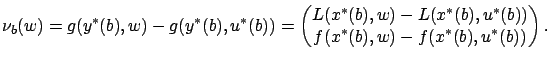
We can thus expand (4.34) as follows:

$$\left\langle\begin{pmatrix} p_0^* \\ p^*(b) \end{pmatrix},\be... ...n{pmatrix} L(x^*(b),u^*(b)) \\ f(x^*(b),u^*(b)) \end{pmatrix}\right\rangle.$$

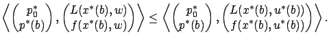
Recalling the expression (4.8) for the Hamiltonian, we see that this is equivalent to

$$H(x^*(b),w,p^*(b),p_0^*)\le H(x^*(b),u^*(b),p^*(b),p_0^*).$$ (4.35)

In the above derivation, $w$ was an arbitrary element of the control set $U$ and $b$ was an arbitrary time in the interval $(t_0,t^*)$ at which the optimal control $u^*$ is continuous. Thus we have established that the Hamiltonian maximization condition holds everywhere except possibly a finite number of time instants (discontinuities of $u^*$ ). Additionally, recall that $u^*$ is piecewise continuous and we adopted the convention (see page ) that the value of a piecewise continuous function at each discontinuity is equal to the limit either from the left or from the right. Letting $b$ in (4.35) approach a discontinuity of $u^*$ or an endpoint of $[t_0,t^*]$ from an appropriate side, and using continuity of $x^*$ and $p^*$ in time and continuity of $H$ in all variables, we see that the Hamiltonian maximization condition must actually hold everywhere.

This conclusion can be understood intuitively as follows. The Hamiltonian is the inner product of the augmented adjoint vector $\Big({\textstyle{p_0^*}\atop \textstyle{p^*}}\Big)$ with the right-hand side of the augmented control system (the velocity of $y$ ). When the optimal control is perturbed, the state trajectory deviates from the optimal one in a direction that makes a nonpositive inner product with the augmented adjoint vector (at the time when the perturbation stops acting). Therefore, such control perturbations can only decrease the Hamiltonian, regardless of the value of the perturbed control during the perturbation interval.