4.2.8 Adjoint equation

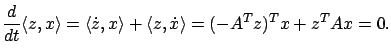
As we already mentioned on page , two (time-varying) linear systems of the form $\dot x=Ax$ and $\dot z=-A^Tz$ are called adjoint to each other. Solutions of adjoint systems are linked by the property that their inner product $\langle z(t),x(t)\rangle$ remains constant, as shown by the following simple calculation:

$$\frac d{dt}\langle z,x\rangle=\langle \dot z,x\rangle+\langle z,\dot x\rangle =(-A^Tz)^Tx+z^TAx=0.$$

We now consider a specific pair of adjoint systems on the time interval $[t_0,t^*]$ . As the first system (the $x$ -system in the above discussion) we take the variational equation (4.19), described in more detail by the equations (4.20) and (4.21). The second, adjoint system is then

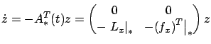$$\dot z=-A_*^T(t)z= \begin{pmatrix}0 & 0\\ -\left.{L}_{x}\right\vert _{*} & -\big.{\left({f}_{x}\right)^T}\big\vert _* \end{pmatrix}z$$ (4.31)

where in the last expression, obtained from (4.21), ${L}_{x}$ is a column vector (it is the gradient of $L$ with respect to $x$ ) and $({{f}_{x}})^T$ is the transpose of the Jacobian matrix of $f$ with respect to $x$ . Let us denote the first component of $z$ by $p_0$ and the vector of the remaining $n$ components of $z$ by $p$ . Then the first differential equation in (4.31) reads $\dot p_0=0$ while the rest of the system (4.31) becomes

$$\dot p =-\left.{L}_{x}\right\vert _{*}p_0-\big.{\left({f}_{x}\right)^T}\big\vert _*p$$

which, in view of the definition (4.2) of the Hamiltonian, is equivalent to

$$\dot p=-{H}_{x}(x^*,u^*,p,p_0).$$

Now, let us specify the terminal condition for the system (4.31) at time $t^*$ by setting $z(t^*)$ equal to the vector (4.28). Further, we relabel the $p$ -component of the solution $z$ corresponding to this terminal condition as $p^*$ . This gives $p_0(t)= p_0^*$ for all $t$ and

$$\dot p^*=-{H}_{x}(x^*,u^*,p^*,p_0^*)$$

which is the second canonical equation in (4.1). With a slight abuse of terminology, we will sometimes refer to this differential equation as the adjoint equation. It is easy to see that the first canonical equation in (4.1) also holds by the definition of $H$ ; thus statement 1 of the maximum principle has been established. By the aforementioned property of adjoint systems, we have

$$\left\langle \begin{pmatrix}{p_0^*}\\ {p^*(t)}\end{pmatrix},\psi(... ...\\ {p^*(t^*)}\end{pmatrix},\psi(t^*)\right\rangle \qquad\forall\, t\in[t_0,t^*]$$ (4.32)

for every solution $\psi$ of the variational equation (4.19).

The vector (4.28), which is normal to the separating hyperplane, is nonzero. Since (4.31) is a homogeneous (unforced) linear time-varying system, we have

$$\begin{pmatrix}p_0^* \\ p^*(t) \end{pmatrix}\ne 0\qquad \forall\,t\in[t_0,t^*]$$ (4.33)

as required in the statement of the maximum principle. Geometrically, we can think of the vector in (4.33) as the normal vector to a hyperplane passing through $y^*(t)$ . We can then associate the solution of the adjoint system to a family of hyperplanes that is ``flowing back" along the optimal trajectory. In view of (4.32), the perturbed trajectory associated with $\psi$ always remains on the same side of the hyperplane.