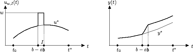
4.2.3 Spatial control perturbation

We now construct control perturbations known as ``needle" perturbations, or Pontryagin-McShane perturbations. As the first name suggests, they will be represented by pulses of short duration; the reason for the second name is that perturbations of this kind were first used by McShane in calculus of variations (see Section 3.1.2) and later adopted by Pontryagin's school for the proof of the maximum principle.

Let $w$ be an arbitrary element of the control set $U$ . Consider the interval $I:=(b-\varepsilon a, b]\subset (t_0,t^*)$ , where $b\ne t^*$ is a point of continuity^4.2 of $u^*$ , $a>0$ is arbitrary, and $\varepsilon >0$ is small. We define the perturbed control

$$u_{w,I}(t):=\begin{cases}u^*(t) \quad&\text{ if }\ t\notin I\\ w\quad&\text{ if }\ t\in I \end{cases}$$

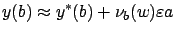
Figure 4.5 illustrates this control perturbation and the resulting state trajectory perturbation. As the figure suggests, the perturbed trajectory $y$ corresponding to $u_{w,I}$ will deviate from $y^*$ on the interval $I$ and afterwards will ``run parallel" to $y^*$ . We now proceed to formally characterize the deviation over $I$ ; the behavior of $y$ over the interval $[b,t^*]$ will be studied in Section 4.2.4.

Figure: A spatial control perturbation and its effect on the trajectory

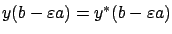
We will let $\approx$ denote equality up to terms of order $o(\varepsilon )$ . The first-order Taylor expansion of $y^*$ around $t=b$ gives

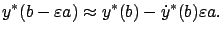$$y^*(b-\varepsilon a)\approx y^*(b) -\dot y^*(b)\varepsilon a.$$ (4.10)

Rearranging terms and using the fact that $y^*$ satisfies the differential equation (4.7) with $u=u^*$ , we have

$$y^*(b)\approx <tex2html_comment_mark>90 y^*(b-\varepsilon a)+g(y^*(b),u^*(b))\varepsilon a.$$ (4.11)

On the other hand, the first-order Taylor expansion of the perturbed solution $y$ around $t=b-\varepsilon a$ yields

$$y(b)\approx y(b-\varepsilon a)+\dot y(b-\varepsilon a)\varepsilon a$$

where by $\dot y(b-\varepsilon a)$ we mean the right-sided derivative of $y$ at $t=b-\varepsilon a$ . Since $y(b-\varepsilon a)=y^*(b-\varepsilon a)$ by construction and $y$ satisfies (4.7) with $u=u_{w,I}$ , we obtain

$$y(b)\approx y^*(b-\varepsilon a)+g(y^*(b-\varepsilon a),w)\varepsilon a.$$ (4.12)

We now apply the Taylor expansion to the last term in (4.12):

$$g(y^*(b-\varepsilon a),w)\varepsilon a \approx g(y^*(b),w)\varepsilon a+ {g}_{y}(y^*(b),w)(y^*(b-\varepsilon a )-y^*(b))\varepsilon a.$$ (4.13)

In view of (4.10), the second term on the right-hand side of (4.13) is of order $\varepsilon ^2$ ; hence we can omit it and the approximation will remain valid. Thus (4.12) simplifies to

$$y(b)\approx y^*(b-\varepsilon a)+ g(y^*(b),w)\varepsilon a.$$

Comparing this formula with (4.11), we arrive at

$$y(b)\approx y^*(b)+\nu_b(w)\varepsilon a$$ (4.14)

where

$$\nu_b(w):=g(y^*(b),w)-g(y^*(b),u^*(b)).$$ (4.15)

Intuitively, this result makes sense: up to terms of order $o(\varepsilon )$ , the difference between the two states $y(b)$ and $y^*(b)$ is the difference (4.15) between the state velocities at $y=y^*(b)$ corresponding to $u=w$ and $u=u^*(b)$ , multiplied by the length $\varepsilon a$ of the time interval on which the perturbation is acting.