Next: 4.2.3 Spatial control perturbation
Up: 4.2 Proof of the
Previous: 4.2.1 From Lagrange to
Contents
Index
4.2.2 Temporal control perturbation
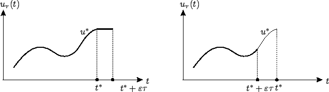
Let us see what happens if we introduce a small
change in the terminal time  of the optimal trajectory, i.e., let the optimal control act on a little
longer or a little shorter time interval. We formalize this as follows: for an arbitrary
of the optimal trajectory, i.e., let the optimal control act on a little
longer or a little shorter time interval. We formalize this as follows: for an arbitrary
 and a small
 , we consider the perturbed
control
, we consider the perturbed
control
which is illustrated by the thick curves in Figure 4.3 (for the
two cases depending on the sign of  ).
).
Figure:
A temporal perturbation
|
|
We are interested in the value of the
resulting perturbed trajectory  at the new terminal time
 . For
. For  , the first-order Taylor expansion of
around
, the first-order Taylor expansion of
around  gives
gives
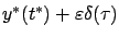
 |
(4.9) |
For  , we have
 and the first-order Taylor expansion of
  around
gives the same result.
The vector
around
gives the same result.
The vector
 describes
the infinitesimal (first-order in
describes
the infinitesimal (first-order in
 ) perturbation
of the terminal point. By
definition,
) perturbation
of the terminal point. By
definition,
 depends linearly on
. As we vary
over
depends linearly on
. As we vary
over
 , keeping
fixed, the points
, keeping
fixed, the points
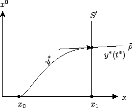
 form a line through
  . We denote
this line by
. We denote
this line by
 ; see Figure 4.4. Every point on
corresponds to a control
; see Figure 4.4. Every point on
corresponds to a control  for
some
. On the other hand, the approximation of
for
some
. On the other hand, the approximation of
 by
is valid only in the limit as
by
is valid only in the limit as
 . So,
tells us the direction--but
not the magnitude--of the terminal point deviation caused by
an infinitesimal change in the terminal time. The arrow
over
. So,
tells us the direction--but
not the magnitude--of the terminal point deviation caused by
an infinitesimal change in the terminal time. The arrow
over  is meant to indicate that points on the line correspond
to perturbation directions. Note that we are describing deviations of the terminal point in the
is meant to indicate that points on the line correspond
to perturbation directions. Note that we are describing deviations of the terminal point in the  -space only, ignoring the differences in the terminal times; accordingly, the time axis is not included in the figures.
Figure:
The effect of a temporal control perturbation
|
|
Next: 4.2.3 Spatial control perturbation
Up: 4.2 Proof of the
Previous: 4.2.1 From Lagrange to
Contents
Index
Daniel
2010-12-20