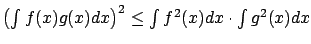
... them.¹

In Tom Stoppard's famous play ``Arcadia" there is an interesting argument between a mathematician and a historian about what is more important: scientific progress or the personalities behind it. In a technical book such as this one, the emphasis is clear, but some flavor of the history can enrich one's understanding and appreciation of the subject.

.
.
.
.
.
.
.
.
.
.
.
.
.
.
.
.
.
.
.
.
.
.
.
.
.
.
.
.
.
.

... product.^1.1

There is no consensus in the literature whether the gradient is a column vector or a row vector. Treating it as a row vector would simplify the notation since it often appears in a product with another vector. Geometrically, however, it plays the role of a regular column vector, and for consistency we follow this latter convention everywhere.

.
.
.
.
.
.
.
.
.
.
.
.
.
.
.
.
.
.
.
.
.
.
.
.
.
.
.
.
.
.

....^1.2

The term $o(\alpha^2)$ can be described more precisely using Taylor's theorem with remainder, which is a higher-order generalization of the Mean Value Theorem; see, e.g., [Rud76, Theorem 5.15]. We will discuss this issue in more detail later when deriving the corresponding result in calculus of variations (see Section 2.6).

.
.
.
.
.
.
.
.
.
.
.
.
.
.
.
.
.
.
.
.
.
.
.
.
.
.
.
.
.
.

... perturbation^1.3

With a slight abuse of terminology, we call $\eta$ a perturbation even though the actual perturbation is $\alpha\eta$ .

.
.
.
.
.
.
.
.
.
.
.
.
.
.
.
.
.
.
.
.
.
.
.
.
.
.
.
.
.
.

... functions^2.1

Actually, the curve in Figure 2.1 is not the graph of a function. There is a tendency to ignore this difference between curves and graphs of functions when formulating calculus of variations problems.

.
.
.
.
.
.
.
.
.
.
.
.
.
.
.
.
.
.
.
.
.
.
.
.
.
.
.
.
.
.

... fact.^2.2

Since we are discussing weak extrema, to accommodate piecewise $\mathcal C^1$ curves we need to slightly generalize the definition of the 1-norm; see Section 3.1.1 for details. Also, the equation (2.23) holds away from the discontinuities of $y'$ . To prove this, we would need to modify the proof of Lemma 2.2 to cover functions $\xi$ that are only piecewise continuous (see page  for a precise definition of this class), while still working with $\eta\in\mathcal C^1$ .

.
.
.
.
.
.
.
.
.
.
.
.
.
.
.
.
.
.
.
.
.
.
.
.
.
.
.
.
.
.

... applied.^2.3

Note that while $\Vert\eta_\varepsilon \Vert _1$ is large for small $\varepsilon$ , once $\varepsilon$ is fixed we have $\Vert\alpha\eta\Vert _1\to 0$ as $\alpha\to 0$ , so the perturbed curves are still close to $y$ in the sense of the 1-norm.

.
.
.
.
.
.
.
.
.
.
.
.
.
.
.
.
.
.
.
.
.
.
.
.
.
.
.
.
.
.

... norm^2.4

I.e., $\left(\int f(x)g(x)dx\right)^2\le \int f^2(x)dx\cdot\int g^2(x)dx$ .

.
.
.
.
.
.
.
.
.
.
.
.
.
.
.
.
.
.
.
.
.
.
.
.
.
.
.
.
.
.

... analysis^3.1

The reader who finds this derivation difficult to follow might wish to skip it at first reading. We also note that the insight gained from solving Exercise 2.6 should be helpful here.

.
.
.
.
.
.
.
.
.
.
.
.
.
.
.
.
.
.
.
.
.
.
.
.
.
.
.
.
.
.

...function!measurablemeasurable^3.2

The class of measurable functions is obtained from that of piecewise continuous functions by taking the closure with respect to almost-everywhere convergence.

.
.
.
.
.
.
.
.
.
.
.
.
.
.
.
.
.
.
.
.
.
.
.
.
.
.
.
.
.
.

...l-dubois-reymond^3.3

That lemma, translated to the present notation, requires $\left.{H}_{u}\right\vert _{*}$ to be continuous; however, it is clear from its proof that piecewise continuity is enough.

.
.
.
.
.
.
.
.
.
.
.
.
.
.
.
.
.
.
.
.
.
.
.
.
.
.
.
.
.
.

...ss-constrained^4.1

The reader might need to revisit that section, as its terminology and notation will be freely used here.

.
.
.
.
.
.
.
.
.
.
.
.
.
.
.
.
.
.
.
.
.
.
.
.
.
.
.
.
.
.

... continuity^4.2

The reason for this assumption is that the subsequent Taylor expansions rely on $y$ being differentiable at $t=b$ .

.
.
.
.
.
.
.
.
.
.
.
.
.
.
.
.
.
.
.
.
.
.
.
.
.
.
.
.
.
.

... itself.^4.3

There is one degenerate case in which we cannot directly apply the Separating Hyperplane Theorem as described, namely, the case when the interior of $C_{t^*}$ is empty. However, it can be shown that if the interior of the convex set $C_{t^*}$ is empty then there exists a hyperplane that contains $C_{t^*}$ (see, e.g., [dlF00, p. 238]), and this hyperplane trivially separates $\vec\mu$ and $C_{t^*}$ .

.
.
.
.
.
.
.
.
.
.
.
.
.
.
.
.
.
.
.
.
.
.
.
.
.
.
.
.
.
.

... time.^4.4

Here and below, when using the notation $\left.\right\vert _{*}$ we also mean that $p_0=p_0^*$ .

.
.
.
.
.
.
.
.
.
.
.
.
.
.
.
.
.
.
.
.
.
.
.
.
.
.
.
.
.
.

... curve^4.5

The shape of the switching curve in the figure is slightly distorted for better visualization; in reality the trajectory converges to 0 faster.

.
.
.
.
.
.
.
.
.
.
.
.
.
.
.
.
.
.
.
.
.
.
.
.
.
.
.
.
.
.

... minimum.^4.6

This situation is to be contrasted with the one in Example 4.4.

.
.
.
.
.
.
.
.
.
.
.
.
.
.
.
.
.
.
.
.
.
.
.
.
.
.
.
.
.
.

...$form$ ^5.1

Note the difference between the previous expression for the minimizing control $u$, which is given pointwise in $t$ and $x$, and the current expression for $u^*$ which is evaluated along the corresponding state trajectory $x^*$. The claim about optimality of $u^*$ is actually somewhat informal at this point, but will be carefully justified very soon (in Section 5.1.4).

.
.
.
.
.
.
.
.
.
.
.
.
.
.
.
.
.
.
.
.
.
.
.
.
.
.
.
.
.
.

... problemproblem.^5.2

For this infinite-horizon problem to be well posed, we need to be sure that the value of the integral 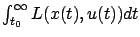$\int_{t_0}^\infty L(x(t),u(t))dt$ is finite at least for some controls. We will investigate this issue in detail for the linear quadratic regulator problem in the next chapter. For now we proceed formally, without worrying about the possibility that the problem might be ill posed.

.
.
.
.
.
.
.
.
.
.
.
.
.
.
.
.
.
.
.
.
.
.
.
.
.
.
.
.
.
.

... equation.^5.3

We note that generalized solution concepts, particularly those relaxing the continuous differentiability requirement, are important in the theory of ordinary differential equations as well. One such solution concept (albeit a very simple one) is provided by the class of absolutely continuous functions, as we discussed in Section 3.3.1.

.
.
.
.
.
.
.
.
.
.
.
.
.
.
.
.
.
.
.
.
.
.
.
.
.
.
.
.
.
.

... subset^5.4

In Sections 5.3.1 and 5.3.2 we could have easily taken the domain of $v$ to be a subset of $\mathbb R^n$ rather than the entire $\mathbb R^n$ .

.
.
.
.
.
.
.
.
.
.
.
.
.
.
.
.
.
.
.
.
.
.
.
.
.
.
.
.
.
.

... linear.^6.1

Of course, the idea that quadratic optimization problems lead to linear update laws goes back to Gauss's least squares method.

.
.
.
.
.
.
.
.
.
.
.
.
.
.
.
.
.
.
.
.
.
.
.
.
.
.
.
.
.
.

...$time.$ ^6.2

It is interesting to digress briefly and note that if we had $R=-1$ then the RDE would be $P=-P^2-1$, which looks very similar but is fundamentally different in that its solutions do not exist globally backward in time (cf. page ). Thus our standing assumption that $R$ is nonnegative is important. We invite the reader to figure out exactly where this assumption comes into play in the preceding argument.

.
.
.
.
.
.
.
.
.
.
.
.
.
.
.
.
.
.
.
.
.
.
.
.
.
.
.
.
.
.

... be^6.3

For consistency with our previous notation, it would have been more accurate to denote the limiting quantities by $V^\infty$ , $u^*_\infty$ , etc. We omit the superscripts and subscripts $\infty$ for simplicity, since we will be focusing on the infinite-horizon problem from now on.

.
.
.
.
.
.
.
.
.
.
.
.
.
.
.
.
.
.
.
.
.
.
.
.
.
.
.
.
.
.

... space^7.1

The use of an asterisk for the dual space is not to be confused with the use of the same symbol throughout the book to indicate optimality.

.
.
.
.
.
.
.
.
.
.
.
.
.
.
.
.
.
.
.
.
.
.
.
.
.
.
.
.
.
.

... matrixHurwitz.^7.2

A matrix is called Hurwitz if all its eigenvalues have negative real parts.

.
.
.
.
.
.
.
.
.
.
.
.
.
.
.
.
.
.
.
.
.
.
.
.
.
.
.
.
.
.

... norms^7.3

See the definition (1.32) on page .

.
.
.
.
.
.
.
.
.
.
.
.
.
.
.
.
.
.
.
.
.
.
.
.
.
.
.
.
.
.