6.2.4 Complete result and discussion

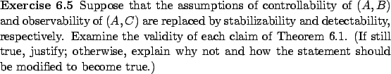
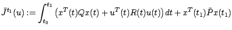
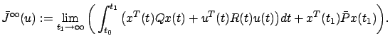
We now collect the results obtained in this section so far, as well as a few additional claims not yet proved, into a single theorem summarizing the solution of the infinite-horizon LQR problem and its main properties.

PROOF (remaining claims). Statement 1 of the theorem was proved in Section 6.2.1 with the exception of two claims: the strict positive definiteness of $P$ (we only showed that $P=P^T\ge 0$ ) and the uniqueness property. Statements 2 and 3 were proved in Section 6.2.2, except for the uniqueness of the optimal control. Statement 4 was proved in Section 6.2.3. With these results in place, we now establish the remaining claims.

Let us first prove that $P>0$ . We already know that $P \ge 0$ . Suppose that $x_0^TPx_0=0$ for some $x_0$ , which in view of statement 2 means that for this initial condition $x_0$ the optimal cost $\int_{t_0}^\infty ((x^*)^T(t) C^TCx^*(t)+(u^*)^T(t)Ru^*(t))dt$ equals 0. This is possible only if $Cx^*\equiv 0$ and $u^*\equiv 0$ (since $R>0$ ). By observability we must then have $x^*\equiv 0$ , as it is well known that the output of an observable linear time-invariant system (with the zero input) can be identically 0 only along the zero trajectory. Thus $x_0=0$ which proves that $P$ is indeed positive definite.

Let us now prove that $P$ is a unique solution of the ARE in the class of positive definite matrices. In fact, we will show that it is unique even in the class of positive semidefinite matrices. Suppose that the ARE has another positive semidefinite solution $\bar P$ . Consider the new cost

$$\bar J^{t_1}(u):=\int_{t_0}^{t_1}\big(x^T(t)Qx(t)+u^T(t)R(t)u(t)\big)dt+x^T(t_1)\bar Px(t_1)$$

and its infinite-horizon counterpart

$$\bar J^{\infty}(u):=\lim_{t_1\to\infty}\bigg( \int_{t_0}^{t_1}\big(x^T(t)Qx(t)+u^T(t)R(t)u(t)\big)dt+x^T(t_1)\bar Px(t_1)\bigg).$$

By statements 4 and 2 of this theorem, the same control $u^*$ as in statement 3 gives

$$\bar J^{\infty}(u^*)=\int_{t_0}^\infty \big((x^*)^T(t)Qx^*(t)+(u^*)^T(t)Ru^*(t)\big)dt=x_0^TPx_0$$

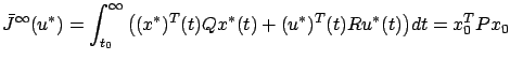
and this is the optimal cost with respect to $\bar J^{\infty}$ because for every other control $u$ we have

$$\bar J^{\infty}(u) \ge \int_{t_0}^{\infty}\big(x^T(t)Qx(t)+u^T(t)R(t)u(t)\big)dt\ge x_0^TPx_0.$$

We also know from the results of Section 6.1 that the optimal cost with respect to $\bar J^{t_1}(u)$ is $x_0^TP(t_0;\bar P,t_1)x_0$ , where $P(t_0;\bar P,t_1)$ denotes the solution at time $t_0$ of the RDE (6.14) with the boundary condition $P(t_1)=\bar P$ . It follows that $P=\lim_{t_1\to\infty} P(t_0;\bar P,t_1)$ , i.e., $P$ is the steady-state solution of the RDE corresponding to $\bar P$ as the terminal condition. But this steady-state solution must be $\bar P$ itself, because $\bar P$ is an equilibrium solution of the RDE (by virtue of satisfying the ARE). Therefore, $\bar P=P$ and the uniqueness property is confirmed.

Finally, to show that the optimal control is unique, recall the equations (5.13) and (5.14) in Section 5.1.3 which say that an optimal control must satisfy

$$u^*(t)=\arg\min_{u\in U}\left\{L(t,x^*(t),u)+\left\langle {V}_{x}(t,x^*(t)),f(t,x^*(t),u)\right\rangle \right\}$$

or, what is the same,

$$u^*(t)=\arg\max_{u\in U} H(t,x^*(t),u,-{V}_{x}(t,x^*(t))).$$

For the infinite-horizon LQR problem and the value function $V(x)=x^TPx$ this condition takes the form

$$u^*(t)=\arg\min_{u\in\mathbb{R}^m}\left\{(x^*)^T(t)Qx^*(t)+u^TRu+ 2(x^*)^T(t)PAx^*(t)+2(x^*)^T(t)PBu\right\}$$

and it is easy to check (cf. Section 6.1.3) that this uniquely identifies the feedback law given in statement 3. 

We can see from the proof that the observability assumption was only used for establishing exponential stability of the optimal closed-loop system (statement 4) and the positive definiteness and uniqueness of $P$ in statement 1 (the uniqueness proof relied on observability indirectly because it invoked statement 4). The controllability assumption, on the other hand, was used for showing the existence of $P$ which is crucial for all the other claims. Nevertheless, there remains the possibility that some or all claims could be proved without relying on these assumptions.

In view of statement 1 of Theorem 6.1 and its proof, we know that the ARE has exactly one positive semidefinite solution $P$ , and this solution is in fact positive definite and gives the optimal cost and optimal control via statements 2 and 3. For example, consider the infinite-horizon version of Example 6.1, with the system $\dot x=u$ and the cost $J(u)=\int_{t_0}^{\infty}(x^2(t)+u^2(t))dt$ . The ARE $P^2-1=0$ has two solutions, $P=\pm 1$ , of which $P=1$ is the one we want. The optimal cost is $V(x_0)=x_0^2$ and the optimal control is $u^*=-x^*$ . The result that the reader obtained in Exercise 6.4 should also immediately yield the optimal cost for that problem and the exponentially stable optimal closed-loop system.

Linearity, time-invariance, and exponential stability are very desirable features of the optimal closed-loop system, indicating that the infinite-horizon LQR problem provides good control design guidelines. The choice of the matrices $Q$ and $R$ is often part of the design process, which helps shape the behavior of the state and the control signal.