We begin by making a series of observations about the behavior of
![]() as a function of
as a function of ![]() , with the goal of establishing that
, with the goal of establishing that
![]() exists (under the additional assumption of controllability) and has some interesting properties. This path will eventually lead us to a complete solution of the infinite-horizon LQR problem.
exists (under the additional assumption of controllability) and has some interesting properties. This path will eventually lead us to a complete solution of the infinite-horizon LQR problem.
MONOTONICITY. It is not hard to see that the finite-horizon optimal cost
![]() is a
monotonically nondecreasing function of the final time
is a
monotonically nondecreasing function of the final time ![]() . Indeed, let
. Indeed, let ![]() . Using (6.25), the definition of the value function, and the standing assumptions that
. Using (6.25), the definition of the value function, and the standing assumptions that ![]() and
and
![]() , we have
, we have
BOUNDEDNESS. It is not true in general that the optimal cost
![]() remains bounded as
remains bounded as
![]() . For example, if the system is
. For example, if the system is ![]() (no control) then its solutions are growing exponentials and the infinite-horizon cost is clearly unbounded. However, we now show that the finite-horizon optimal cost
(no control) then its solutions are growing exponentials and the infinite-horizon cost is clearly unbounded. However, we now show that the finite-horizon optimal cost
![]() remains bounded as
remains bounded as
![]() assuming that
assuming that
![]() is a controllable pair.
Indeed, controllability guarantees the existence of a time
is a controllable pair.
Indeed, controllability guarantees the existence of a time ![]() and a control
and a control ![]() that steers the state
from
that steers the state
from ![]() at time
at time ![]() to 0 at time
to 0 at time ![]() . After time
. After time ![]() , set
, set ![]() equal to 0.
This control yields a state trajectory
equal to 0.
This control yields a state trajectory ![]() satisfying
satisfying
![]() for all
for all
![]() , and we have
, and we have
Since the above integral does not depend on
![[*]](crossref.gif) where its necessity will be re-examined).
where its necessity will be re-examined).
EXISTENCE OF THE LIMIT. From the previous two claims it immediately follows that
![]() has a limit as
has a limit as
![]() .
It turns out that more is true, namely,
the matrix
.
It turns out that more is true, namely,
the matrix
![]() is well defined. To see why, let us consider some specific initial conditions
is well defined. To see why, let us consider some specific initial conditions ![]() (we can do this because all the facts established so far are valid for arbitrary
(we can do this because all the facts established so far are valid for arbitrary ![]() ). First, let
). First, let ![]() with
with ![]() as defined on page for some
as defined on page for some
![]() . Then
. Then
![]() ,
implying that each diagonal entry of
,
implying that each diagonal entry of
![]() has a limit as
has a limit as
![]() . Next,
let
. Next,
let
![]() for some
for some ![]() . Recalling that
. Recalling that
![]() is symmetric (Exercise 6.2), we have
is symmetric (Exercise 6.2), we have
![]() , from which we can deduce that the off-diagonal entries of
, from which we can deduce that the off-diagonal entries of
![]() converge as well. We can think of
converge as well. We can think of
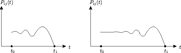
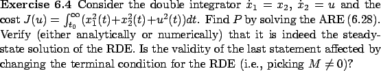
![]() as the solution of the RDE (6.14) that, starting from the zero matrix, has flown backward for infinite time and reached steady state; Figure 6.1 should help visualize this situation.
as the solution of the RDE (6.14) that, starting from the zero matrix, has flown backward for infinite time and reached steady state; Figure 6.1 should help visualize this situation.
PROPERTIES OF THE LIMIT. Since the RDE (6.14) is now a time-invariant differential equation, its solution
![]() actually depends only on the difference
actually depends only on the difference ![]() . Thus it is clear that the steady-state solution
. Thus it is clear that the steady-state solution
![]() , whose existence we just established, does not depend on
, whose existence we just established, does not depend on ![]() , i.e., it is a constant matrix.
Denoting it simply by
, i.e., it is a constant matrix.
Denoting it simply by ![]() , we have
, we have