1.1 Optimal control problem

We begin by describing, very informally and in general terms, the class of optimal control problems that we want to eventually be able to solve. The goal of this brief motivational discussion is to fix the basic concepts and terminology without worrying about technical details.

The first basic ingredient of an optimal control problem is a control system. It generates possible behaviors. In this book, control systems will be described by ordinary differential equations (ODEs) of the form

$$\dot x=f(t,x,u),\qquad x(t_0)=x_0$$ (1.1)

where $x$ is the state taking values in $\mathbb{R}^n$ , $u$ is the control input taking values in some control set $U\subset \mathbb{R}^m$ , $t$ is time, $t_0$ is the initial time, and $x_0$ is the initial state. Both $x$ and $u$ are functions of $t$ , but we will often suppress their time arguments.

The second basic ingredient is the cost functional. It associates a cost with each possible behavior. For a given initial data $(t_0,x_0)$ , the behaviors are parameterized by control functions $u$ . Thus, the cost functional assigns a cost value to each admissible control. In this book, cost functionals will be denoted by $J$ and will be of the form

$$J(u):=\int_{t_0}^{t_f} L(t,x(t),u(t))dt+K(t_f,x_f)$$ (1.2)

where $L$ and $K$ are given functions (running cost and terminal cost, respectively), $t_f$ is the final (or terminal) time which is either free or fixed, and $x_f:=x(t_f)$ is the final (or terminal) state which is either free or fixed or belongs to some given target set. Note again that $u$ itself is a function of time; this is why we say that $J$ is a functional (a real-valued function on a space of functions).

The optimal control problem can then be posed as follows: Find a control $u$ that minimizes $J(u)$ over all admissible controls (or at least over nearby controls). Later we will need to come back to this problem formulation and fill in some technical details. In particular, we will need to specify what regularity properties should be imposed on the function $f$ and on the admissible controls $u$ to ensure that state trajectories of the control system are well defined. Several versions of the above problem (depending, for example, on the role of the final time and the final state) will be stated more precisely when we are ready to study them. The reader who wishes to preview this material can find it in Section 3.3.

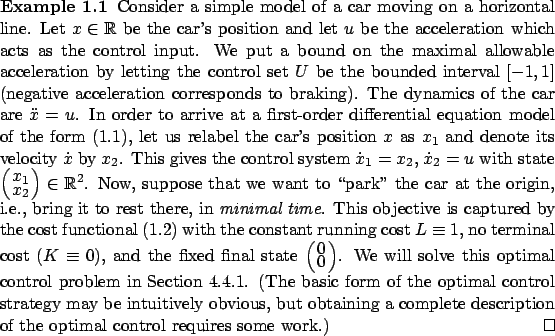
It can be argued that optimality is a universal principle of life, in the sense that many--if not most--processes in nature are governed by solutions to some optimization problems (although we may never know exactly what is being optimized). We will soon see that fundamental laws of mechanics can be cast in an optimization context. From an engineering point of view, optimality provides a very useful design principle, and the cost to be minimized (or the profit to be maximized) is often naturally contained in the problem itself. Some examples of optimal control problems arising in applications include the following:

• Send a rocket to the moon with minimal fuel consumption;
• Produce a given amount of chemical in minimal time and/or with minimal amount of catalyst used (or maximize the amount produced in given time);
• Bring sales of a new product to a desired level while minimizing the amount of money spent on the advertising campaign;
• Maximize communication throughput or accuracy for a given channel bandwidth/capacity.

The reader will easily think of other examples. Several specific optimal control problems will be examined in detail later in the book. We briefly discuss one simple example here to better illustrate the general problem formulation.

In this book we focus on the mathematical theory of optimal control. We will not undertake an in-depth study of any of the applications mentioned above. Instead, we will concentrate on the fundamental aspects common to all of them. After finishing this book, the reader familiar with a specific application domain should have no difficulty reading papers that deal with applications of optimal control theory to that domain, and will be prepared to think creatively about new ways of applying the theory.

We can view the optimal control problem as that of choosing the best path among all paths feasible for the system, with respect to the given cost function. In this sense, the problem is infinite-dimensional, because the space of paths is an infinite-dimensional function space. This problem is also a dynamic optimization problem, in the sense that it involves a dynamical system and time. However, to gain appreciation for this problem, it will be useful to first recall some basic facts about the more standard static finite-dimensional optimization problem, concerned with finding a minimum of a given function $f:\mathbb{R}^n\to\mathbb{R}$ . Then, when we get back to infinite-dimensional optimization, we will more clearly see the similarities but also the differences.

The subject studied in this book has a rich and beautiful history; the topics are ordered in such a way as to allow us to trace its chronological development. In particular, we will start with calculus of variations, which deals with path optimization but not in the setting of control systems. The optimization problems treated by calculus of variations are infinite-dimensional but not dynamic. We will then make a transition to optimal control theory and develop a truly dynamic framework. This modern treatment is based on two key developments, initially independent but ultimately closely related and complementary to each other: the maximum principle and the principle of dynamic programming.