2.2.1 Weak and strong extrema

We recall from Section 1.3 that in order to define local optimality, we must first select a norm, and on the space of $\mathcal C^1$ curves $y:[a,b]\to\mathbb{R}$ there are two natural candidates for the norm: the 0-norm (1.30) and the 1-norm (1.31). Extrema (minima and maxima) of $J$ with respect to the 0-norm are called strong extrema, and those with respect to the 1-norm are called weak extrema.

These two notions will be central to our subsequent developments, and so it is useful to reflect on them for a little while until the distinction between the two types of extrema becomes clear and there is no possibility of confusing them. If a $\mathcal C^1$ curve $y^*$ is a strong extremum, then it is automatically a weak one, but the converse is not true. The reason is that an $\varepsilon$ -ball around $y^*$ with respect to the 0-norm contains the $\varepsilon$ -ball with respect to the 1-norm for the same $\varepsilon$ , as is clear from the norm definitions; on the other hand, the $\varepsilon$ -ball with respect to the 1-norm does not contain the $\varepsilon '$ -ball with respect to the 0-norm for any $\varepsilon '$ , no matter how small. In other words, it is harder to satisfy $J(y^*)\le J(y)$ for all $y$ close enough to $y^*$ if we understand closeness in the sense of the 0-norm. Closeness in the sense of the 1-norm is a more restrictive condition, since the derivatives of $y$ and $y^*$ also have to be close, meaning that there are fewer perturbations to check than for the 0-norm. We will see that, for the same reason, studying weak extrema is easier than studying strong extrema.

On the other hand, it will become evident later that the concept of a weak minimum is not very suitable in optimal control. Indeed, an optimal trajectory $y^*$ should give a lower cost than all nearby trajectories $y$ , and there is no compelling reason to take into account the difference between the derivatives of $y^*$ and $y$ . Also, as we already mentioned, requiring $y$ to be a $\mathcal C^1$ curve is often too restrictive. Specifically, we will want to allow curves $y$ which are continuous everywhere on $[a,b]$ and whose derivative $y'$ exists everywhere except possibly a finite number of points in $[a,b]$ and is continuous and bounded between these points. Let us agree to call such curves piecewise $\mathcal C^1$ , to reflect the fact that they are concatenations of finitely many $\mathcal C^1$ pieces. (We could define the class of admissible curves more precisely using the notion of an absolutely continuous function; we will revisit this issue in Section 3.3 as we make the transition to optimal control.) If we use the 0-norm, then it makes no difference whether $y$ is $\mathcal C^1$ or piecewise $\mathcal C^1$ or just $\mathcal C^0$ ; this is another advantage of the 0-norm over the 1-norm.

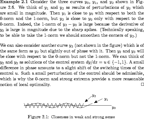
In view of the above remarks, it seems natural to first obtain some basic tools for studying weak minima and then proceed to develop more advanced tools for investigating strong minima. This is essentially what we will do. The next example illustrates some of the points that we just made regarding the 0-norm versus the 1-norm. The exercise that follows should help the reader to better grasp the concepts of weak and strong minima; it is to be solved using only the definitions.