5.1.1 Motivation: the discrete problem

The dynamic programming approach is quite general, but to fix ideas we first present it for the purely discrete case. Consider a system of the form

$$x_{k+1}=f(x_k,u_k),\qquad k=0,1,\dots, T-1$$

where $x_k$ lives in a finite set $X$ consisting of $N$ elements, $u_k$ lives in a finite set $U$ consisting of $M$ elements, and $T,N,M$ are fixed positive integers. We suppose that each possible transition from some $x_k$ to $x_{k+1}$ corresponding to some control value $u_k$ has a cost assigned to it, and there is also a terminal cost function on $X$ . For each trajectory, the total cost accumulated at time $T$ is the sum of the transition costs at time steps $0,\dots,T-1$ plus the terminal cost at $x_T$ . For a given initial state $x_0$ we want to minimize this total cost, the terminal state $x_T$ being free.

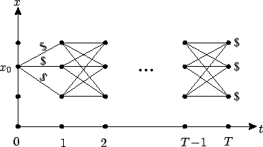
The most naive approach to this problem is as follows: starting from $x_0$ , enumerate all possible trajectories going forward up to time $T$ , calculate the cost for each one, then compare them and select the optimal one. Figure 5.1 provides a visualization of this scenario. It is easy to estimate the computational effort required to implement such a solution: there are $M^T$ possible trajectories and we need $T$ additions to compute the cost for each one, which results in roughly $O(M^TT)$ algebraic operations.

Figure: Discrete case: going forward

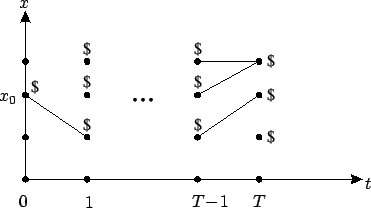
We now examine an alternative approach, which might initially appear counterintuitive: let us go backward in time. At $k=T$ , terminal costs are known for each $x_k$ . At $k=T-1$ , for each $x_k$ we find to which $x_{k+1}$ we should jump so as to have the smallest cost (the one-step running cost plus the terminal cost). Write this optimal ``cost-to-go" next to each $x_k$ and mark the selected path (see Figure 5.2). In case of more than one path giving the same cost, choose one of them at random. Repeat these steps for $k=T-2,\dots, 0$ , working with the costs-to-go computed previously in place of the terminal costs.

Figure: Discrete case: going backward

We claim that when we are done, we will have generated an optimal trajectory from each $x_0$ to some $x_T$ . The justification of this claim relies on the principle of optimality, an observation that we already made during the proof of the maximum principle (see page ). In the present context this principle says that for each time step $k$ , if $x_k$ is a point on an optimal trajectory then the remaining decisions (from time $k$ onward) must constitute an optimal policy with respect to $x_k$ as the initial condition. What the principle of optimality does for us here is guarantee that the paths we discard going backward cannot be portions of optimal trajectories. On the other hand, in the previous approach (going forward) we are not able to discard any paths until we reach the terminal time and finish the calculations.

Let us assess the computational effort associated with this backward scheme. At each time $k$ , for each state $x_k$ and each control $u_k$ we need to add the cost of the corresponding transition to the cost-to-go already computed for the resulting $x_{k+1}$ . Thus, the number of required operations is $O(N MT)$ . Comparing this with the $O(M^TT)$ operations needed for the earlier forward scheme, we conclude that the backward computation is more efficient for large $T$ , with $N$ and $M$ fixed. Of course, the number of operations will still be large if $N$ and $M$ are large (this is the ``curse of dimensionality").

Actually, the above comparison is not really accurate because the backward scheme provides much more information: it finds the optimal policy for every initial condition $x_0$ , and in fact it tells us what the optimal decision is at every $x_k$ for all $k$ . We can restate this last property as follows: the backward scheme yields the optimal control policy in the form of a state feedback law. In the forward scheme, on the other hand, to handle all initial conditions we would need $O(NM^TT)$ operations, and we would still not cover all states $x_k$ for $k>0$ ; hence, a state feedback is not obtained. We see that the backward scheme fulfills the objective formulated in Bellman's quote at the beginning of this chapter. This recursive scheme serves as an example of the general method of dynamic programming.