Consider the system
We know that the dynamics of the double integrator (4.47) are equivalently described by the state-space equations
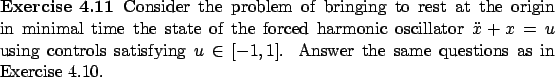
 must
satisfy the adjoint equation
must
satisfy the adjoint equation
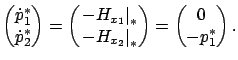
Next, from the Hamiltonian maximization condition and the fact that ![]() we have
we have
![[*]](crossref.gif) ) that
) that
We conclude that the optimal
control ![]() takes only the values
takes only the values ![]() and switches
between these values at most once. Interpreted
in terms of bringing a car to rest
at the origin, the optimal control strategy consists in
switching between
maximal acceleration and maximal braking. The initial sign and the
switching time of course depend on the initial condition. The property that
and switches
between these values at most once. Interpreted
in terms of bringing a car to rest
at the origin, the optimal control strategy consists in
switching between
maximal acceleration and maximal braking. The initial sign and the
switching time of course depend on the initial condition. The property that ![]() only switches
between the extreme values
only switches
between the extreme values ![]() is intuitively natural and
important; such controls are called bang-bang.
is intuitively natural and
important; such controls are called bang-bang.
It turns out that for the present problem, the pattern identified
above uniquely determines the optimal control law for every
initial condition. To see this, let us plot the solutions of the
system (4.47) in the
![]() -plane for
-plane for
![]() . For
. For ![]() , repeated integration gives
, repeated integration gives
![]() and then
and then
![]() for some constants
for some constants ![]() and
and ![]() . The resulting
relation
. The resulting
relation
![]() (where
(where ![]() ) defines a
family of parabolas in the
) defines a
family of parabolas in the
![]() -plane parameterized by
-plane parameterized by
![]() . Similarly, for
. Similarly, for
![]() we obtain the family of parabolas
we obtain the family of parabolas
![]() ,
,
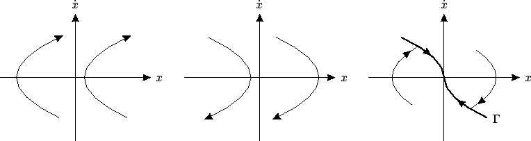
![]() . These curves are shown in
Figure 4.15(a,b), with the
arrows indicating the direction in which they are traversed. It is
easy to see that only two of these trajectories hit the origin
(which is the prescribed final point). Their union is the thick
curve in Figure 4.15(c), which we call the
switching curve and denote by
. These curves are shown in
Figure 4.15(a,b), with the
arrows indicating the direction in which they are traversed. It is
easy to see that only two of these trajectories hit the origin
(which is the prescribed final point). Their union is the thick
curve in Figure 4.15(c), which we call the
switching curve and denote by ![]() ; it is defined by the relation
; it is defined by the relation
![]() . The optimal control
strategy thus consists in applying
. The optimal control
strategy thus consists in applying ![]() or
or ![]() depending on
whether the initial point is below or above
depending on
whether the initial point is below or above ![]() , then
switching the control value exactly on
, then
switching the control value exactly on ![]() and subsequently
following
and subsequently
following ![]() to the origin; no switching is needed if the
initial point is already on
to the origin; no switching is needed if the
initial point is already on ![]() . (Thinking slightly
differently, we can generate all possible optimal
trajectories--which cover the entire plane--by starting at the
origin and flowing backward in time, first following
. (Thinking slightly
differently, we can generate all possible optimal
trajectories--which cover the entire plane--by starting at the
origin and flowing backward in time, first following ![]() and
then switching at an arbitrary point on
and
then switching at an arbitrary point on ![]() .) Recalling the
interpretation of our problem as that of parking a car using
bounded acceleration/braking, the reader can easily relate the
optimal trajectories in the
.) Recalling the
interpretation of our problem as that of parking a car using
bounded acceleration/braking, the reader can easily relate the
optimal trajectories in the
![]() -plane with the
corresponding motions of the car along the
-plane with the
corresponding motions of the car along the ![]() -axis. Note that if
the car is initially moving away from the origin, then it begins
braking until it stops, turns around, and starts accelerating
(this is a ``false" switch because
-axis. Note that if
the car is initially moving away from the origin, then it begins
braking until it stops, turns around, and starts accelerating
(this is a ``false" switch because ![]() actually remains constant),
and then
actually remains constant),
and then ![]() switches sign and the car starts braking again.
switches sign and the car starts braking again.
 |
The optimal control law that we just found has two important
features. First, as we already said, it is bang-bang. Second, we
see that it can be described in the form of a state feedback
law. This is interesting because in general, the maximum principle only provides an
open-loop description of an optimal control; indeed, ![]() depends, besides the state
depends, besides the state ![]() , on the costate
, on the costate ![]() , but
we managed to eliminate this latter dependence here. It is natural
to ask for what more general classes of systems time-optimal
controls have these two properties, i.e., are bang-bang and take
the state feedback form. The bang-bang property will be examined
in detail in the next two subsections. The problem of representing
optimal controls as state feedback laws is rather intricate and
will not be treated in this book, except for the two exercises
below.
, but
we managed to eliminate this latter dependence here. It is natural
to ask for what more general classes of systems time-optimal
controls have these two properties, i.e., are bang-bang and take
the state feedback form. The bang-bang property will be examined
in detail in the next two subsections. The problem of representing
optimal controls as state feedback laws is rather intricate and
will not be treated in this book, except for the two exercises
below.
The next exercise is along the same lines but the solution is less obvious.