


Next: 4.2 Proof of the
Up: 4.1 Statement of the
Previous: 4.1.1 Basic fixed-endpoint control
Contents
Index
4.1.2 Basic variable-endpoint control problem
The Basic Variable-Endpoint Control Problem is the
same as the Basic Fixed-Endpoint Control Problem except the target
set is now of the form
 , where
 is a
is a  -dimensional surface in
 for some nonnegative integer
 . As in Section 1.2.24.1 we define such a surface via
equality constraints:
. As in Section 1.2.24.1 we define such a surface via
equality constraints:
where  ,
,
 are
are
 functions from
to
functions from
to
 . We also
assume that every
. We also
assume that every  is a regular point.
As two extreme special cases,
for
is a regular point.
As two extreme special cases,
for  we obtain
 (which gives a free-time, free-endpoint problem)
while for
(which gives a free-time, free-endpoint problem)
while for  the surface
reduces either to a single point (as in the
Basic Fixed-Endpoint Control Problem) or to a set consisting of isolated points.
The difference between the maximum principle for this problem and the previous
one lies
only in the boundary conditions for the system of canonical equations.
the surface
reduces either to a single point (as in the
Basic Fixed-Endpoint Control Problem) or to a set consisting of isolated points.
The difference between the maximum principle for this problem and the previous
one lies
only in the boundary conditions for the system of canonical equations.
Maximum Principle for the
Basic Variable-Endpoint Control Problem
Let
![$ u^*:[t_0,t_f]\to U$](img978.gif) be an optimal control
and let
be an optimal control
and let
![$ x^*:[t_0,t_f]\to\mathbb{R}^n$](img979.gif) be the
corresponding optimal state trajectory. Then there
exist a function
be the
corresponding optimal state trajectory. Then there
exist a function
![$ p^*:[t_0,t_f]\to\mathbb{R}^n$](img980.gif) and a constant
and a constant
 satisfying
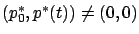 for all
![$ t\in[t_0,t_f]$](img983.gif) and having the following
properties:
and having the following
properties:
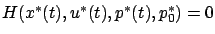
 and
and  satisfy the canonical equations (4.1)
with respect to the Hamiltonian (4.2)
with the boundary conditions
satisfy the canonical equations (4.1)
with respect to the Hamiltonian (4.2)
with the boundary conditions
 and
and
 .
.
-
 for all
and all
for all
and all  .
.
-
 for all
.
for all
.
- The vector
 is orthogonal to the tangent space to
at
is orthogonal to the tangent space to
at  :
:
 |
(4.3) |
The additional necessary condition (4.3)
is called the transversality condition (we encountered its loose
analog in
Example 2.4 and Exercise 2.6 in Section 2.3.5).
We know from Section 1.2.2
that the tangent space can be characterized as
 |
(4.4) |
and that (4.3) is equivalent to saying that
is a linear combination of the gradient vectors
 ,
. Note that
when
and hence
, the transversality condition
reduces to
,
. Note that
when
and hence
, the transversality condition
reduces to
 (because the tangent space is the entire
). On the other hand, the previous version of the maximum
principle is a special case of the present result: when
(because the tangent space is the entire
). On the other hand, the previous version of the maximum
principle is a special case of the present result: when
 , its tangent space is 0 and (4.3)
is true for all
. In general, here as well as in the
Basic Fixed-Endpoint Control Problem, we have
, its tangent space is 0 and (4.3)
is true for all
. In general, here as well as in the
Basic Fixed-Endpoint Control Problem, we have  boundary
conditions imposed on
boundary
conditions imposed on  at
at  and
more at
and
more at  . This gives the correct
total number of boundary conditions
to specify a solution of the
. This gives the correct
total number of boundary conditions
to specify a solution of the  -dimensional system (4.1).
However, in the Basic Fixed-Endpoint Control Problem
was fixed
and
was free, while here
we have
degrees of freedom for
but only
-dimensional system (4.1).
However, in the Basic Fixed-Endpoint Control Problem
was fixed
and
was free, while here
we have
degrees of freedom for
but only
 degrees of freedom for
 .
We see that the freer the state, the less free the costate: each
additional degree of freedom for
eliminates one degree of
freedom for
.
.
We see that the freer the state, the less free the costate: each
additional degree of freedom for
eliminates one degree of
freedom for
.
The maximum principle was developed by the Pontryagin school in the Soviet Union in the late 1950s. It was presented to the wider research community
at the first IFAC World Congress in Moscow in 1960 and in the celebrated
book [PBGM62]. It is worth reflecting that the developments we have covered
so far in this book--starting
from the Euler-Lagrange equation, continuing to the Hamiltonian formulation, and culminating
in the maximum principle--span more
than 200 years. The progress made during this time period is quite remarkable,
yet the origins of the maximum principle are clearly traceable to the early work in calculus of variations.
Next: 4.2 Proof of the
Up: 4.1 Statement of the
Previous: 4.1.1 Basic fixed-endpoint control
Contents
Index
Daniel
2010-12-20