To better understand the behavior of ![]() as a function of
as a function of ![]() along the
optimal trajectory, let us
bring in the second variation.
To do this, we must first augment the description (3.25) of the perturbed state trajectory with the second-order term in
along the
optimal trajectory, let us
bring in the second variation.
To do this, we must first augment the description (3.25) of the perturbed state trajectory with the second-order term in ![]() , writing
, writing
![]() We then need to go back to the
expressions (3.32)-(3.34) and expand them by adding
second-order terms in
We then need to go back to the
expressions (3.32)-(3.34) and expand them by adding
second-order terms in ![]() . With
. With ![]() already set equal to
already set equal to ![]() as defined above,
it is relatively straightforward to check that the
as defined above,
it is relatively straightforward to check that the ![]() -dependent terms drop out--exactly in the same way as the
-dependent terms drop out--exactly in the same way as the ![]() -dependent terms dropped out of the first variation (3.35)--and that the second variation is given by
-dependent terms dropped out of the first variation (3.35)--and that the second variation is given by
![]()
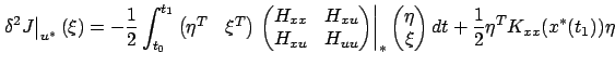
We know from
the second-order necessary condition for optimality (see
Section 1.3.3) that we must have
![]() for all
for all ![]() .
Let us concentrate
on the integrand in (3.41) and ask the following question:
does one term in the Hessian matrix of
.
Let us concentrate
on the integrand in (3.41) and ask the following question:
does one term in the Hessian matrix of ![]() dominate the other terms? If
yes, then this term should be nonpositive to ensure the correct sign of
dominate the other terms? If
yes, then this term should be nonpositive to ensure the correct sign of
![]() .
We encountered a very similar issue in Section 2.6.1 in relation to the
inequality (2.61). We found there that for the overall
integral to be nonnegative, the function multiplying
.
We encountered a very similar issue in Section 2.6.1 in relation to the
inequality (2.61). We found there that for the overall
integral to be nonnegative, the function multiplying
![]() must be nonnegative, because
must be nonnegative, because ![]() may be large while
may be large while ![]() itself is small. The present situation is a bit different since
itself is small. The present situation is a bit different since ![]() is not
just the derivative of
is not
just the derivative of ![]() , i.e., the system relating the two is not
a simple integrator. However, the corresponding conclusion is still valid:
, i.e., the system relating the two is not
a simple integrator. However, the corresponding conclusion is still valid:
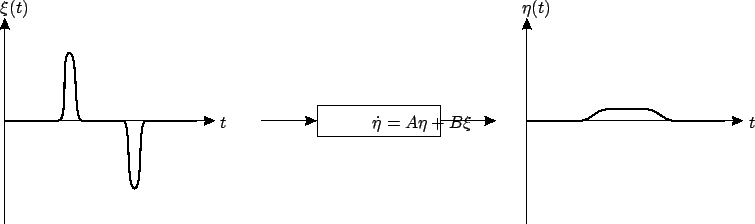
![]() is the dominant term because we may have a large
is the dominant term because we may have a large
![]() producing a small
producing a small ![]() (but not vice versa), as illustrated in Figure 3.5.
Thus, in order for the second variation (3.41)
to be nonnegative, we must have
(but not vice versa), as illustrated in Figure 3.5.
Thus, in order for the second variation (3.41)
to be nonnegative, we must have
![]() for all
for all ![]() , which can only happen if the matrix
, which can only happen if the matrix
![]() is negative semidefinite:
is negative semidefinite:
We already know from (3.39) that for each
![]() , the function
, the function
![]() must
have a stationary point at
must
have a stationary point at ![]() . Now the
Legendre-Clebsch condition (3.42) tells us that if this stationary
point is an extremum, then it is necessarily a maximum.
Even though we have not proved that the stationary point must
indeed be an extremum, it is tempting to conjecture that this
Hamiltonian maximization property is true. In other words, our
findings up to this point are very suggestive of the following
(not yet proved) necessary conditions for
optimality: If
. Now the
Legendre-Clebsch condition (3.42) tells us that if this stationary
point is an extremum, then it is necessarily a maximum.
Even though we have not proved that the stationary point must
indeed be an extremum, it is tempting to conjecture that this
Hamiltonian maximization property is true. In other words, our
findings up to this point are very suggestive of the following
(not yet proved) necessary conditions for
optimality: If
![]() is an optimal control and
is an optimal control and
![]() is the corresponding optimal state trajectory, then
there exists an adjoint vector (costate)
is the corresponding optimal state trajectory, then
there exists an adjoint vector (costate)
![]() such
that:
such
that: