5.3.3 HJB equation and the value function

Let us finally go back to our fixed-time optimal control problem from Section 5.1.2 and its HJB equation (5.10) with the boundary condition (5.3), with the goal of resolving the difficulty identified at the end of Section 5.2.1. Specifically, our hope is that the value function (5.2) is a solution of the HJB equation in the viscosity sense. In order to more closely match the PDE (5.34), we first rewrite the HJB equation as

$$-{V}_{t}(t,x)-\inf_{u\in U} \left\{L(t,x,u)+\left\langle {V}_{x}(t,x),f(t,x,u)\right\rangle \right\}=0.$$ (5.34)

As we saw in the previous subsection, flipping the sign in a PDE affects its viscosity solutions; it will turn out that the above sign convention is the correct one. The PDE (5.38) is still not in the form (5.34) because it contains the additional independent variable $t$ . However, the concepts and results of Sections 5.3.1 and 5.3.2 extend to this time-space setting without difficulties. Alternatively, we can absorb $t$ into $x$ by introducing the extra state variable $x_{n+1}:=t$ , a trick already familiar to us from Chapters 3 and 4. Then the PDE (5.38) takes the form (5.34) with the obvious definition of the function $F$ , except that the domain of $v$ is the subset^5.4 $[t_0,t_1]\times \mathbb{R}^n$ of $\mathbb{R}^{n+1}$ . The control $u$ does not appear as an argument of $F$ since the definition of $F$ includes taking the infimum over $u$ .

Now the theory of viscosity solutions can be applied to the HJB equation. Under suitable technical assumptions on the functions $f$ , $L$ , and $K$ , we have the following main result: The value function $V$ is a unique viscosity solution of the HJB equation (5.38) with the boundary condition (5.3). It is also locally Lipschitz (but, as we know from Section 5.2.1, not necessarily $\mathcal C^1$ ). Regarding the technical assumptions, we will not list them here (see the references in Section 5.4) but we mention that they are satisfied if, for example, $f$ , $L$ , and $K$ are uniformly continuous, ${f}_{x}$ , ${L}_{x}$ , and ${K}_{x}$ are bounded, and $U$ is a compact set.

We will not attempt to establish the uniqueness and the Lipschitz property, but we do want to understand why $V$ is a viscosity solution of (5.38). To this end, let us prove that $V$ is a viscosity subsolution. The additional technical assumptions cited above are actually not needed for this claim. Fix an arbitrary pair $(t_0,x_0)$ . We need to show that for every $\mathcal C^1$ test function $\varphi=\varphi(t,x)$ such that $\varphi-V$ attains a local minimum at $(t_0,x_0)$ , the inequality

$$-\varphi_t(t_0,x_0)-\inf_{u\in U}\{ L(t_0,x_0,u)+\langle \varphi_x(t_0,x_0), f(t_0,x_0,u)\rangle \}\le 0$$

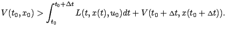
must be satisfied. Suppose that, on the contrary, there exist a $\mathcal C^1$ function $\varphi$ and a control value $u_0\in U$ such that

$$\varphi(t_0,x_0)=V(t_0,x_0),\qquad \varphi(t,x)\ge V(t,x)\quad \forall\,(t,x) (t_0,x_0)$$ (5.35)

and

$$-\varphi_t(t_0,x_0)-L(t_0,x_0,u_0)-\langle \varphi_x(t_0,x_0), f(t_0,x_0,u_0)\rangle > 0.$$ (5.36)

Taking $(t_0,x_0)$ as the initial condition, let us consider the state trajectory $x(\cdot)$ that results from applying the control $u\equiv u_0$ on a small time interval $[t_0,t_0+{\scriptstyle\Delta}t]$ . We will now demonstrate that the rate of change of the value function along this trajectory is inconsistent with the principle of optimality. As long as we pick ${\scriptstyle\Delta}t$ to be sufficiently small, we have

$$V(t_0 +{\scriptstyle\Delta}t,x(t_0+{\scriptstyle\Delta}t))-V(t_0,x_0)\l... ...lta}t))-\varphi(t_0,x_0)=\int_{t_0}^{t_0+\Delta t}\frac{d}{dt}\varphi(t,x(t))dt$$

$$=\int_{t_0}^{t_0+\Delta t} \big(\varphi_t(t,x(t))+\langle \varphi... ...(t)), f(t,x(t),u_0)\rangle \big) dt < -\int_{t_0}^{t_0+\Delta t}L(t,x(t),u_0)dt$$

where the first inequality is a direct consequence of (5.39) and the last inequality follows from (5.40) by virtue of continuity of all the functions appearing there. We thus obtain

$$V(t_0,x_0)>\int_{t_0}^{t_0+\Delta t}L(t,x(t),u_0)dt+V(t_0+{\scriptstyle\Delta}t,x(t_0+{\scriptstyle\Delta}t)).$$ (5.37)

On the other hand, the principle of optimality (5.4) tells us that

$$V(t_0,x_0)\le \int_{t_0}^{t_0+\Delta t} L(t,x(t),u_0)dt+V(t_0+{\scriptstyle\Delta}t,x(t_0+{\scriptstyle\Delta} t))$$

and we arrive at a contradiction. Provided that optimal controls exist, here is a slightly different way to see why (5.41) cannot be true: it would imply that the optimal cost-to-go from $(t_0,x_0)$ is higher than the cost of applying the constant control $u\equiv u_0$ on $[t_0,t_0+{\scriptstyle\Delta}t]$ followed by an optimal control on the remaining interval $(t_0+{\scriptstyle\Delta}t,t_1]$ , which is clearly impossible.

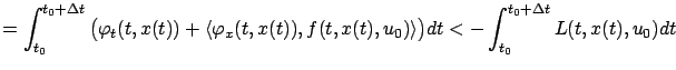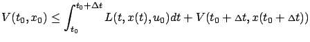We now have at our disposal a more rigorous formulation of the necessary conditions for optimality from Section 5.1.3. The above reasoning is of course quite different from our original derivation of the HJB equation, but we see that the principle of optimality still plays a central role. The sufficient condition for optimality from Section 5.1.4 can also be generalized, a task that we leave as an exercise.